In general, if we want to shoot random numbers filling in a normalized probability distribution $P(y)$, the random numbers $y$ can be calculated by the inverse function of integral of the $P(y)$, $F^{-1}(x)$, where $F(x)=\int_{-\infty}^x P(t) dt$ and $x$ is an uniform random variable with the range of $0 < x <1$. Therefore, in order to shoot $y$ filling in a normal (Gaussian) distribution $f(x;\mu,\sigma^2) = \frac{1}{\sigma\sqrt{2\pi}}e^{-\frac{(x-\mu)^2}{2\sigma^2}}$, $y$ can be calculated by the inverse function of the integral of the normal distribution, $F^{-1}(x)$. Based on the calculations below, $F^{-1}(x)$ is described as \begin{align} y = F^{-1}(x) = \sqrt{2}\sigma\ \mathrm{erf}^{-1}\left(2x - 1\right) + \mu, \end{align} where $ 0 < x < 1$. Fortunately, the ROOT has an implementation of the inverse error function $\mathrm{erf}^{-1}$ (TMath::ErfInverse()), and thus the random numbers filling in the normal distribution $f(x;\mu,\sigma^2)$ can be shot by “mean+sigma*sqrt(2)*TMath::ErfInverse(2*rndm-1)”. In the formula, “rndm” is an uniform random number in (0,1).

At first, we have to obtain the integral of the normal (Gaussian) distribution $f(t;\mu,\sigma^2)$, $F(x)$. The integral $F(x)$ can be written as \begin{align} F(x) = \int_{-\infty}^x f(t;\mu,\sigma^2) dt = \frac{1}{2}\left[1+\mathrm{erf}\left(\frac{y-\mu}{\sqrt{2}\sigma}\right)\right], \end{align} where $ 0 < F(y) < 1$. The derivation is the following. Assuming $T=\frac{t-\mu}{\sqrt{2}\sigma}$, $\sqrt{2}\sigma dT = dt$, and \begin{align} F(x) &= \int_{-\infty}^x f(t;\mu,\sigma^2) dt\\ & = \frac{1}{\sigma\sqrt{2\pi}}\int_{-\infty}^{x}e^{-\frac{(t-\mu)^2}{2\sigma^2}}dt\\ & = \frac{1}{\sigma\sqrt{2\pi}}\int_{-\infty}^{\frac{x-\mu}{\sqrt{2}\sigma}} e^{-T^2} \sqrt{2}\sigma dT\\ & = \frac{1}{\sqrt{\pi}}\int_{-\infty}^{\frac{x-\mu}{\sqrt{2}\sigma}} e^{-T^2} dT\\ & = \frac{1}{\sqrt{\pi}}\int_{-\infty}^{0} e^{-T^2} dT + \frac{1}{\sqrt{\pi}}\int_{0}^{\frac{x-\mu}{\sqrt{2}\sigma}} e^{-T^2} dT\\ & = \frac{1}{2}\left[-\frac{2}{\sqrt{\pi}}\int_{0}^{-\infty} e^{-T^2} dT+\frac{2}{\sqrt{\pi}}\int_{0}^{\frac{x-\mu}{\sqrt{2}\sigma}} e^{-T^2} dT\right]. \end{align} Since $\mathrm{erf}(x) = \dfrac{2}{\sqrt{\pi}}\displaystyle\int_0^x e^{-t^2}dt$ and $\mathrm{erf}(-\infty) = \dfrac{2}{\sqrt{\pi}}\displaystyle\int_0^{-\infty} e^{-t^2}dt = -1$, finally we get \begin{align} F(x) = \frac{1}{2}\left[1+\mathrm{erf}\left(\frac{x-\mu}{\sqrt{2}\sigma}\right)\right]. \end{align} By the way, $F(x)$ can vary in $ 0 < F(x) < 1$, because $\mathrm{erf}(x)$ can vary in $-1 < \mathrm{erf}(x) < 1$. (In fact, this is trivial, because the $f(x;\mu,\sigma^2)$ is a probability distribution and should be larger than 0. In addition, the integral of the $f(x;\mu,\sigma^2)$ is normalized to 1.)

Then the inverse function of the integral of the normal distribution, $F^{-1}(x)$, can be obtained as below. From $F(x) = \frac{1}{2}\left[1+\mathrm{erf}\left(\frac{x-\mu}{\sqrt{2}\sigma}\right)\right]$, \begin{align} \mathrm{erf}\left(\frac{x-\mu}{\sqrt{2}\sigma}\right) &= 2F(x) - 1\\ \Rightarrow \mathrm{erf}^{-1}\left[\mathrm{erf}\left(\frac{x-\mu}{\sqrt{2}\sigma}\right)\right] &= \mathrm{erf}^{-1}\left[2F(x) - 1\right]\\ \Rightarrow \frac{x-\mu}{\sqrt{2}\sigma} &= \mathrm{erf}^{-1}\left[2F(x) - 1\right]\\ \Rightarrow x &= \sqrt{2}\sigma\ \mathrm{erf}^{-1}\left[2F(x) - 1\right] + \mu. \end{align} As a result, the inverse function of the integral of the normal distribution is \begin{align} y=F^{-1}(x) = \sqrt{2}\sigma\ \mathrm{erf}^{-1}\left(2x - 1\right) + \mu, \end{align} where $x$ can vary in $ 0 < x < 1$.

“Computation of the error function erf(x). Erf(x) = (2/sqrt(pi)) Integral(exp(-t^2))dt between 0 and x”

In TeX format, $\mathrm{erf}(x) = \dfrac{2}{\sqrt{\pi}}\displaystyle\int_0^x e^{-t^2}dt$

“returns the inverse error function, x must be -1<x<1”

“Periodicity = 2**31, generates a number in (0,1).”

$f(x;\mu,\sigma^2) = \frac{1}{\sigma\sqrt{2\pi}}e^{-\frac{(x-\mu)^2}{2\sigma^2}}$

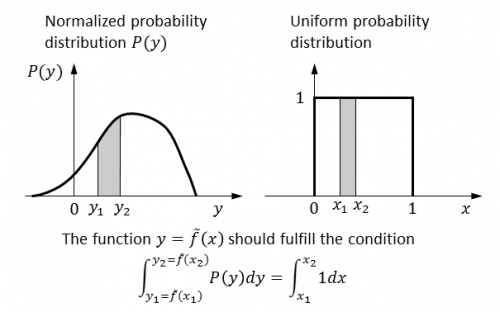
A random variable $y$ filling in a given normalized probability distribution $P(t)$ can be calculated from an uniform random variable $x$ ($0<x<1$). The function $\tilde{f}(x)$ to transform $x$ to $y$ is described as \begin{align} y&=\tilde{f}(x)=F^{-1}(x),\\ F(y)&=\int_{-\infty}^y P(t)dt, \end{align} where $F^{-1}(x)$ is an inverse function of $F(y)$.