Garfield++ software#

Garfield++ is a physics software toolkit for the simulation of the particle detectors based on ionization, such as gaseous detectors and semiconductor detectors.

Example 1: The Grand Raiden VDC#

The Grand Raiden spectrometer at RCNP has two vertical drift chambers which act as focal plane detectors. Some of the basic properties of the drift chamber can be found in the table below.

Gas mixture	Ar (71%) + iC4H10 (29%) + isopropyl-alcohol
Effective area	115 cm (W) x 12 cm (H)
Anode-Cathode Gap	10 mm
Potential wire spacing	2 mm
Anode wire spacing	6 mm
Cathode plate voltage	-0 V
Anode wire voltage	-5,600 V
Potential wire voltage	-300 V
Anode wire size	20 um
Potential wire size	50 um

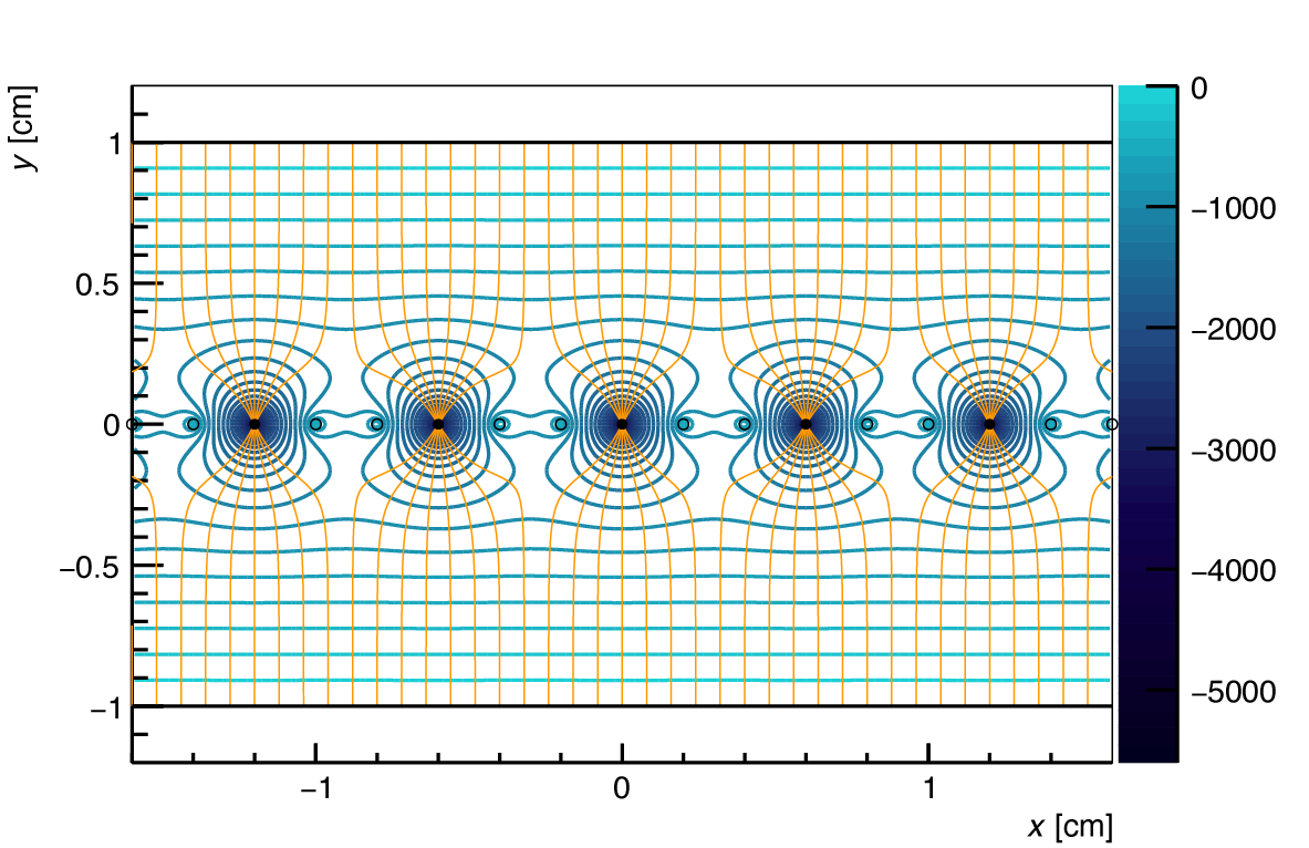
Visualizing the field lines#

It’s useful to visualize the field in a VDC, to understand the drift region for electrons & ions, and also to understand where the electron avalanche occurs. The example (compiled by referring to Garfield++ example code AnalyticField/fieldlines.py, and the 2D wire chamber example) given below demonstrates this.

First we initialize.

import ROOT
ROOT.gSystem.Load("libGarfield")

ROOT.Garfield.plottingEngine.SetPalette(ROOT.kDeepSea)
canvas = ROOT.TCanvas("fieldCanvas", "Electric Field", 1200, 800)

Then we define the gas mixture.

gas = ROOT.Garfield.MediumMagboltz("Ar", 71.0, "isobutane", 29.0)
gas.SetTemperature(293.15)  # Room temperature in K
gas.SetPressure(760.0)      # Torr
gas.Initialise(True)

cmp = ROOT.Garfield.ComponentAnalyticField()
cmp.SetMedium(gas)

Then we define the layout of each VDC cell.

gap = 1 # distance between the cathodes and the row of wires [cm]
ds = 0.0020 # anode (sense) wire diameter [cm]
da = 0.0050 # potential wire diameter [cm]
vs = -5600. # anode wire voltage
vg = -300. # potential wire voltage
period = 0.2 # wire spacing [cm].

# Define the placement of the two cathode plates
cmp.AddPlaneY(gap,  0.0, "cathode top")
cmp.AddPlaneY(gap*(-1),  0.0, "cathode bottom")
# Add the wires
cmp.AddWire(0, 0, ds, vs, "anode")
cmp.AddWire(0.2, 0, da, vg, "potential")
cmp.AddWire(0.4, 0, da, vg, "potential")
# Set the repetition period
cmp.SetPeriodicityX(period*3)
cmp.PrintCell()

First let’s add the potential lines. If you want to plot here, just add the ines in step 7 (i.e fieldView.PlotContour() and canvas.SaveAs("name.pdf")).

xmin, xmax = -8 * period, 8 * period # in cm
ymin, ymax = -1.2, 1.2 # in cm

fieldView.SetArea(xmin, ymin, xmax, ymax)
fieldView.SetVoltageRange(0, -5600)
fieldView.SetNumberOfContours(40)

Next add the field lines. Here I have manually assigned the seeds of the field lines, since the automatic assignment by fieldView.EqualFluxIntervals() didn’t work well.

# Plot field lines for y > 0 cm
xf1 = ROOT.std.vector('double')()
yf1 = ROOT.std.vector('double')()
zf1 = ROOT.std.vector('double')()

# Plot field lines for y < 0 cm
xf2 = ROOT.std.vector('double')()
yf2 = ROOT.std.vector('double')()
zf2 = ROOT.std.vector('double')()

n = 40

for i in range(n):
    x = xmin + i*(xmax - xmin)/n
    xf1.push_back(x)
    yf1.push_back(1)  # fixed y
    zf1.push_back(0.0)  # fixed z

for i in range(n):
    x = xmin + i*(xmax - xmin)/n
    xf2.push_back(x)
    yf2.push_back(-1)  # fixed y
    zf2.push_back(0.0)  # fixed z

Next add the VDC cell.

cellView = ROOT.Garfield.ViewCell(cmp)
cellView.SetCanvas(fieldView.GetCanvas())
cellView.SetArea(xmin, ymin, xmax, ymax)

Finally plot the potential lines, field lines and the VDC cell and save.

fieldView.PlotContour()
fieldView.PlotFieldLines(xf1, yf1, zf1, False, False)
fieldView.PlotFieldLines(xf2, yf2, zf2, False, False)
cellView.Plot2d()
canvas.SaveAs("GR_VDC_FieldLines4.pdf")

The image should turn out like this.

Estimating the capacitance#

On this page