ヒストグラムファイルを作成する
tree->Draw()はいろいろな相関を見れる良い方法ですが、決まった相関を複数確認したい時(シフト業務など)には向いていません。
そこでここではTTreeProjectionProcessorを使ってあらかじめヒストグラムを定義しておく方法を紹介します。
この手法の良いとして以下のようなものが挙げられます。
- 複数の相関を短時間で確認できること
- 解析中に逐次相関を確認できること
- 操作が簡単のでシフト業務などに有用
さて、TTreeProjectionProcessorの使い方ですが、別のyamlファイルにてヒストグラムの定義をする必要があります。
ここでは、二体反応のシミュレーションを使います。
まず、以下のようにヒストグラムを定義していきます。ここではhist/TwoBodyReaction.hist.yamlという名前にしておきます。
alias:
ScatThetaCM: mctruth[2].Theta()*TMath::RadToDeg()
scatEx: mctruth[2].fE-mctruth[2].TKE()-mctruth[0].M()
recoilTKE: recoil.TKE()
recoilThetaLab: recoil.Theta()*TMath::RadToDeg()
pmag: TMath::Sqrt( recoil.Px()*recoil.Px() + recoil.Py()*recoil.Py() + recoil.Pz()*recoil.Pz() )
qprojxy: TMath::Sqrt(pmag*pmag-recoil.Pz()*recoil.Pz())/197
qz: recoil.Pz()/197
group:
- name: monte_carlo_simulation
title: Monte-Carlo Simulation ( Two Body Reaction)
contents:
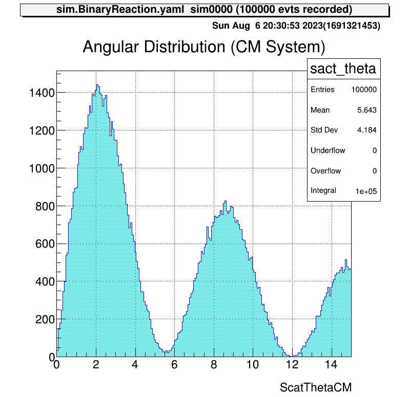
- name: sact_theta
title: Angular Distribution (CM System)
x: ["ScatThetaCM", 200, 0.0, 15.0]
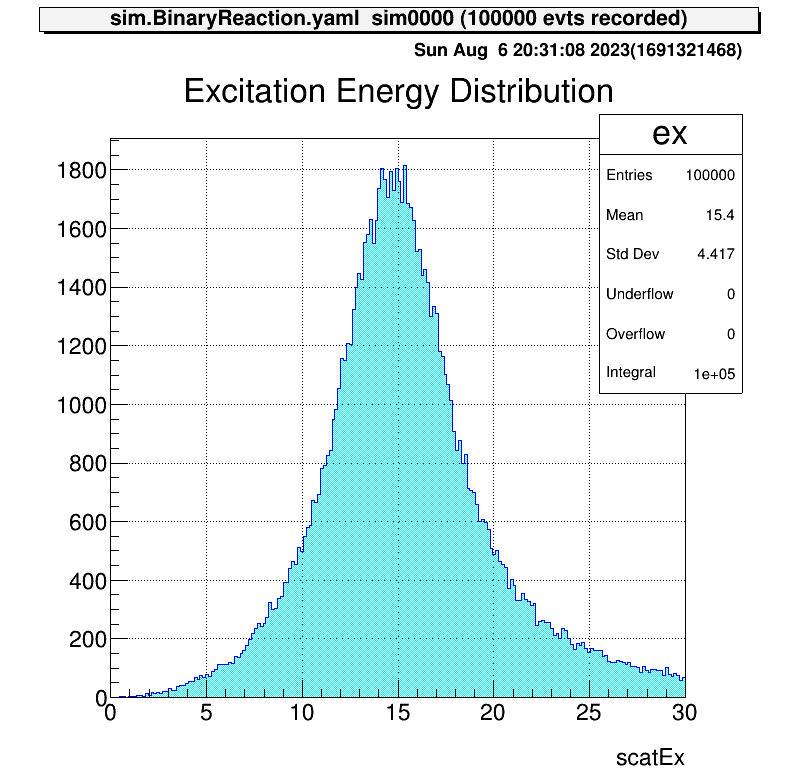
- name: ex
title: Excitation Energy Distribution
x: ["scatEx", 200, 0., 30.]
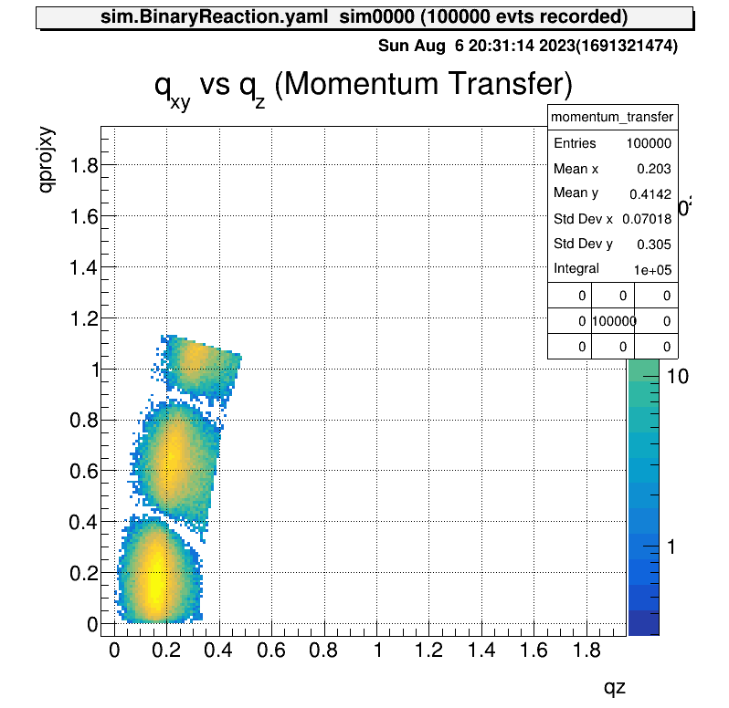
- name: momentum_transfer
title: q_{xy} vs q_{z} (Momentum Transfer)
x: ["qz", 200, -0.05, 1.95]
y: ["qprojxy", 200,-0.05, 1.95]
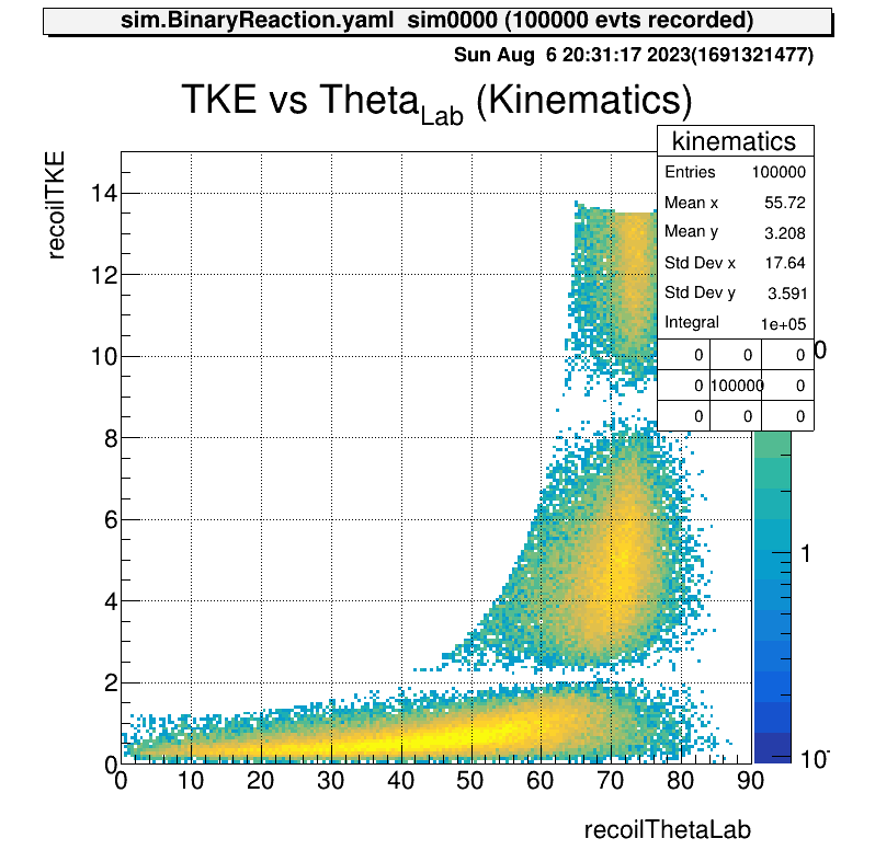
- name: kinematics
title: TKE vs Theta_{Lab} (Kinematics)
x: ["recoilThetaLab", 200, 0, 90]
y: ["recoilTKE", 200, 0, 15]group:でヒストグラムのグループを定義し、contents:以降の- name:にてヒストグラムを定義します。
一次元ならx:のみ、二次元ならx:、y:をマッピングします。リストの中身は[描画したいデータ、Bin数、最小値、最大値]です。
そのほかにもゲートをかける(cut:)や次元の違う配列の比較を行う(async:)などのオプションがあります。
このようにして作成したyamlファイルを以下のように追加してあげればOKです。(ここではsteering/TwoBodyReactionWithHistogram.yaml内に書きます。。)
Anchor:
  - &maxevt 100000
  - &histout output/sim/TwoBodyReactionWithHistogram.hist.root
  - &output output/sim/TwoBodyReactionWithHistogram.root
Processor:
  - name: timer
    type: art::TTimerProcessor
##################################################################################################
  - name: MyTProcessor
    type: art::TBinaryReactionGenerator
    parameter:
      AngDistFile: ""  # [TString] file name of the angular distribution. The format of content is '%f %f'.
      AngMom: 0  # [Int_t] angular momentum for bessel function. If -1 (default), the isotopic distribution is assumed.
      AngRange: [0, 15]  # [FloatVec_t] the range of angular distribution
      DoRandomizePhi: 1  # [Int_t] Flag to randomize phi direction (uniform)
      ExMean: 15  # [Float_t] mean of excitation energy
      ExRange: [0, 30]  # [FloatVec_t] the range of excitation energy
      ExWidth: 7  # [Float_t] width of excitation energy : default is delta function
      KinMean: 100  # [Float_t] mean kinetic energy per nucleon
      MCTruthCollection: mctruth  # [TString] output name of MC truth
      MaxLoop: *maxevt  # [Int_t] the maximum number of loop
      OutputCollection: recoil  # [TString] output name of particle array
      OutputTransparency: 0  # [Bool_t] Output is persistent if false (default)
      Particle1: [86, 36]  # [IntVec_t] mass and atomic number for particle1
      Particle2: [2, 1]  # [IntVec_t] mass and atomic number for particle2
      Particle3: [86, 36]  # [IntVec_t] mass and atomic number for particle3
      RunName: sim  # [TString] run name
      RunNumber: 0  # [Int_t] run number
      Verbose: 1  # [Int_t] verbose level (default 1 : non quiet)
##################################################################################################
  - name: projectiontpccorrelation
    type: art::TTreeProjectionProcessor
    parameter:
      Type: art::TTreeProjection
      FileName: hist/TwoBodyReaction.hist.yaml
      OutputFilename: *histout
##################################################################################################
  - name: MyTOutputTreeProcessor
    type: art::TOutputTreeProcessor
    parameter:
      FileName: *output  # [TString] The name of output file
      OutputTransparency: 0  # [Bool_t] Output is persistent if false (default)
      SplitLevel: 0  # [Int_t] Split level of tree defined in TTree (default is changed to be 0)
      TreeName: tree  # [TString] The name of output tree
      Verbose: 1  # [Int_t] verbose level (default 1 : non quiet)
##################################################################################################これまで同様に、該当のyamlファイルを読み込ませ、解析します。やり方はここ
正しく解析できていれば以下のディレクトリができているはずです。
artemis [4] ls

 artemis
>   0 TH2F hseed           hseed
    1 art::TTreeProjGroup monte_carlo_simulation Monte-Carlo Simulation ( Two Body Reaction)
    2 art::TAnalysisInfo analysisInfo
1番のディレクトリにhist.yamlで定義してヒストグラムが入っています。以下のコマンドで中身のリストを表示できます。
artemis [5] cd 1
artemis [6] ls

 monte_carlo_simulation
>   0 art::TH1FTreeProj sact_theta      Angular Distribution (CM System)
    1 art::TH1FTreeProj ex              Excitation Energy Distribution
    2 art::TH2FTreeProj momentum_transfer q_{xy} vs q_{z} (Momentum Transfer)
    3 art::TH2FTreeProj kinematics      TKE vs Theta_{Lab} (Kinematics)
あとは以下のコマンドなどで描画できます。
zone 2 2
ht 0:3 colz
正しく書けていれば以下のような図ができます。
| 重心系散乱角度 | 励起エネルギー分布 | 運動量移行 | 運動学 |
|---|---|---|---|
|
|
|
|